Predictive Modeling Kaggle Challenge

Purpose

This is my second data science project at Lambda School where I participated in a week-long private Kaggle Challenge to predict the functonality of water pumps in Tanzania. For the record, I did not place in the top half of my class but I was able to predict a respectible accuracy by using an XGBoost classification model with both randomized search cross-validation and grid search cross-validation techniques.

This was a really fun challenge because I was able to practically apply concepts that I have learned at Lambda School with real-world data that can be used for social good.

Continue reading if you dare to know more about my journey!

Tanzanian Water Pump Kaggle Challenge Overview

Tanzania Water Pump

Predict which water pumps are faulty.

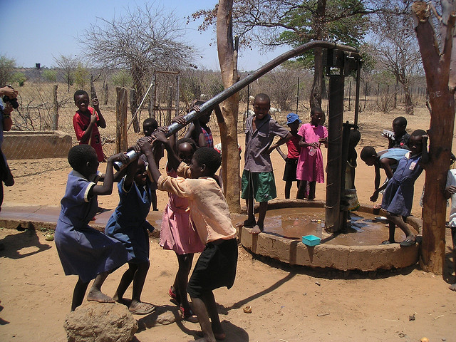
Using data from Taarifa and the Tanzanian Ministry of Water, can you predict which pumps are functional, which need some repairs, and which don’t work at all? Predict one of these three classes based on a number of variables about what kind of pump is operating, when it was installed, and how it is managed. A smart understanding of which waterpoints will fail can improve maintenance operations and ensure that clean, potable water is available to communities across Tanzania.

This predictive modeling challenge comes from DrivenData, an organization who helps non-profits by hosting data science competitions for social impact. The competition has open licensing: “The data is available for use outside of DrivenData.” We are reusing the data on Kaggle’s InClass platform so we can run a weeklong challenge just for your Lambda School Data Science cohort.

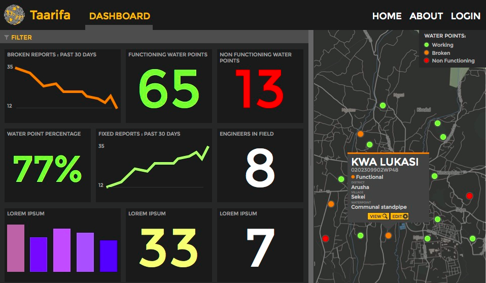
The data comes from the Taarifa waterpoints dashboard, which aggregates data from the Tanzania Ministry of Water. In their own words:

Taarifa is an open source platform for the crowd sourced reporting and triaging of infrastructure related issues. Think of it as a bug tracker for the real world which helps to engage citizens with their local government. We are currently working on an Innovation Project in Tanzania, with various partners.

Taarifa Dashboard

Go here to get the complete Kaggle challenge info.

Tanzanian Water Pump Kaggle Challenge

Importing the Data and an Overloaded Toolbox

I started with retrieving the data from Kaggle like this:

!kaggle competitions download -c ds3-predictive-modeling-challenge

I then imported all of the Python Library tools that I thoughtI might need to use for this project. It turned out that I only used a few of them. But hey, better to be prepared for anything than for nothing.

# Loading potential tools needed not all are used
%matplotlib inline
import eli5
from eli5.sklearn import PermutationImportance
import matplotlib.pyplot as plt
import numpy as np
import pandas as pd
from sklearn.model_selection import train_test_split
import category_encoders as ce
from scipy.stats import randint
from sklearn.model_selection import RandomizedSearchCV
from xgboost import XGBClassifier
from xgboost import XGBRegressor
from sklearn.metrics import roc_auc_score
from sklearn.model_selection import cross_val_score
from pdpbox.pdp import pdp_isolate, pdp_plot
from pdpbox.pdp import pdp_interact, pdp_interact_plot
import shap
from sklearn.metrics import mean_absolute_error
from sklearn.feature_selection import f_regression, SelectKBest
from sklearn.linear_model import Ridge
from sklearn.pipeline import make_pipeline
from sklearn.preprocessing import RobustScaler
from sklearn.preprocessing import StandardScaler
from sklearn.metrics import accuracy_score
from sklearn.impute import SimpleImputer
from sklearn.preprocessing import MinMaxScaler
from sklearn.ensemble import RandomForestRegressor
from sklearn.tree import DecisionTreeRegressor
from sklearn.tree import DecisionTreeClassifier
from sklearn.metrics import f1_score
from sklearn.linear_model import LogisticRegression

Examming the Dataset

The data came pre-split as test_features.csv.zip, train_features.csv.zip, and train_labels.csv.zip files. Here is my quick examination of the data imported.

train_features = pd.read_csv('/home/seek/Documents/GitHub/DS-Project-2---Predictive-Modeling-Challenge/train_features.csv.zip')
pd.options.display.max_columns = 40
train_features.head()

	id	amount_tsh	date_recorded	funder	gps_height	installer	longitude	latitude	wpt_name	num_private	basin	subvillage	region	region_code	district_code	lga	ward	population	public_meeting	recorded_by	scheme_management	scheme_name	permit	construction_year	extraction_type	extraction_type_group	extraction_type_class	management	management_group	payment	payment_type	water_quality	quality_group	quantity	quantity_group	source	source_type	source_class	waterpoint_type	waterpoint_type_group
0	69572	6,000	2011-03-14	Roman	1,390	Roman	34.938…	-9.856…		False	Lake Nyasa	Mnyusi B	Iringa	11	5	Ludewa	Mundindi	109	True	GeoData Consultants Ltd	VWC	Roman	False	1,999	gravity	gravity	gravity	vwc	user-group	pay annually	annually	soft	good	enough	enough	spring	spring	groundwater	communal standpipe	communal standpipe
1	8776	0	2013-03-06	Grumeti	1,399	GRUMETI	34.699…	-2.147…	Zahanati	False	Lake Victoria	Nyamara	Mara	20	2	Serengeti	Natta	280	NaN	GeoData Consultants Ltd	Other	NaN	True	2,010	gravity	gravity	gravity	wug	user-group	never pay	never pay	soft	good	insufficient	insufficient	rainwater harvesting	rainwater harvesting	surface	communal standpipe	communal standpipe
2	34310	25	2013-02-25	Lottery Club	686	World vision	37.461…	-3.821…	Kwa Mahundi	False	Pangani	Majengo	Manyara	21	4	Simanjiro	Ngorika	250	True	GeoData Consultants Ltd	VWC	Nyumba ya mungu pipe scheme	True	2,009	gravity	gravity	gravity	vwc	user-group	pay per bucket	per bucket	soft	good	enough	enough	dam	dam	surface	communal standpipe multiple	communal standpipe
3	67743	0	2013-01-28	Unicef	263	UNICEF	38.486…	-11.155…	Zahanati Ya Nanyumbu	False	Ruvuma / Southern Coast	Mahakamani	Mtwara	90	63	Nanyumbu	Nanyumbu	58	True	GeoData Consultants Ltd	VWC	NaN	True	1,986	submersible	submersible	submersible	vwc	user-group	never pay	never pay	soft	good	dry	dry	machine dbh	borehole	groundwater	communal standpipe multiple	communal standpipe
4	19728	0	2011-07-13	Action In A	0	Artisan	31.131…	-1.825…	Shuleni	False	Lake Victoria	Kyanyamisa	Kagera	18	1	Karagwe	Nyakasimbi	0	True	GeoData Consultants Ltd	NaN	NaN	True	0	gravity	gravity	gravity	other	other	never pay	never pay	soft	good	seasonal	seasonal	rainwater harvesting	rainwater harvesting	surface	communal standpipe	communal standpipe

train_labels = pd.read_csv('/home/seek/Documents/GitHub/DS-Project-2---Predictive-Modeling-Challenge/train_labels.csv.zip')

train_labels.head()

	id	status_group
0	69572	functional
1	8776	functional
2	34310	functional
3	67743	non functional
4	19728	functional

test_features = pd.read_csv('/home/seek/Documents/GitHub/DS-Project-2---Predictive-Modeling-Challenge/test_features.csv.zip')
pd.options.display.max_columns = 40
test_features.head()

	id	amount_tsh	date_recorded	funder	gps_height	installer	longitude	latitude	wpt_name	num_private	basin	subvillage	region	region_code	district_code	lga	ward	population	public_meeting	recorded_by	scheme_management	scheme_name	permit	construction_year	extraction_type	extraction_type_group	extraction_type_class	management	management_group	payment	payment_type	water_quality	quality_group	quantity	quantity_group	source	source_type	source_class	waterpoint_type	waterpoint_type_group
0	50785	0	2013-02-04	Dmdd	1,996	DMDD	35.291…	-4.060…	Dinamu Secondary School	False	Internal	Magoma	Manyara	21	3	Mbulu	Bashay	321	True	GeoData Consultants Ltd	Parastatal	NaN	True	2012	other	other	other	parastatal	parastatal	never pay	never pay	soft	good	seasonal	seasonal	rainwater harvesting	rainwater harvesting	surface	other	other
1	51630	0	2013-02-04	Government Of Tanzania	1,569	DWE	36.657…	-3.309…	Kimnyak	False	Pangani	Kimnyak	Arusha	2	2	Arusha Rural	Kimnyaki	300	True	GeoData Consultants Ltd	VWC	TPRI pipe line	True	2,000	gravity	gravity	gravity	vwc	user-group	never pay	never pay	soft	good	insufficient	insufficient	spring	spring	groundwater	communal standpipe	communal standpipe
2	17168	0	2013-02-01	NaN	1,567	NaN	34.768…	-5.004…	Puma Secondary	False	Internal	Msatu	Singida	13	2	Singida Rural	Puma	500	True	GeoData Consultants Ltd	VWC	P	NaN	2,010	other	other	other	vwc	user-group	never pay	never pay	soft	good	insufficient	insufficient	rainwater harvesting	rainwater harvesting	surface	other	other
3	45559	0	2013-01-22	Finn Water	267	FINN WATER	38.058…	-9.419…	Kwa Mzee Pange	False	Ruvuma / Southern Coast	Kipindimbi	Lindi	80	43	Liwale	Mkutano	250	NaN	GeoData Consultants Ltd	VWC	NaN	True	1,987	other	other	other	vwc	user-group	unknown	unknown	soft	good	dry	dry	shallow well	shallow well	groundwater	other	other
4	49871	500	2013-03-27	Bruder	1,260	BRUDER	35.006…	-10.950…	Kwa Mzee Turuka	False	Ruvuma / Southern Coast	Losonga	Ruvuma	10	3	Mbinga	Mbinga Urban	60	NaN	GeoData Consultants Ltd	Water Board	BRUDER	True	2,000	gravity	gravity	gravity	water board	user-group	pay monthly	monthly	soft	good	enough	enough	spring	spring	groundwater	communal standpipe	communal standpipe

Assigning training and test variables

X_train = train_features
X_test = test_features
y_train = train_labels['status_group']

Getting initial label counts

y_train.value_counts(normalize=True)

functional                 0.543081
non functional             0.384242
functional needs repair    0.072677
Name: status_group, dtype: float64

First Baseline Model Prediction

Now it is time to really get things moving with our first baseline model

Let’s start by assigning our features and target variables.

features = X_train.columns.tolist()
target = y_train

X = features
y = target

XGBoost Classification with RandomizedSearchCV

Now that everything is set, we will build and run the first baseline model and see what happens.

encoder = ce.OrdinalEncoder()
X_train = encoder.fit_transform(X_train)

param_distributions = {
    'n_estimators': randint(50, 300), 
    'max_depth': randint(2, 4)
}

# n_iter & cv parameters are low here so the example runs faster
search = RandomizedSearchCV(
    estimator=XGBClassifier(n_jobs=-1, random_state=42), 
    param_distributions=param_distributions, 
    n_iter=50, 
    scoring='accuracy', 
    n_jobs=-1, 
    cv=2, 
    verbose=10, 
    return_train_score=True, 
    random_state=42
)

search.fit(X_train, y_train)

Fitting 2 folds for each of 50 candidates, totalling 100 fits
[Parallel(n_jobs=-1)]: Using backend LokyBackend with 12 concurrent workers.
[Parallel(n_jobs=-1)]: Done   1 tasks      | elapsed:    8.8s
[Parallel(n_jobs=-1)]: Done   8 tasks      | elapsed:   23.5s
[Parallel(n_jobs=-1)]: Done  17 tasks      | elapsed:   46.4s
[Parallel(n_jobs=-1)]: Done  26 tasks      | elapsed:  1.4min
[Parallel(n_jobs=-1)]: Done  37 tasks      | elapsed:  1.6min
[Parallel(n_jobs=-1)]: Done  48 tasks      | elapsed:  2.4min
[Parallel(n_jobs=-1)]: Done  61 tasks      | elapsed:  2.7min
[Parallel(n_jobs=-1)]: Done  74 tasks      | elapsed:  3.3min
[Parallel(n_jobs=-1)]: Done  88 out of 100 | elapsed:  3.8min remaining:   31.2s
[Parallel(n_jobs=-1)]: Done 100 out of 100 | elapsed:  4.3min finished

RandomizedSearchCV(cv=2, error_score='raise-deprecating',
                   estimator=XGBClassifier(base_score=0.5, booster='gbtree',
                                           colsample_bylevel=1,
                                           colsample_bytree=1, gamma=0,
                                           learning_rate=0.1, max_delta_step=0,
                                           max_depth=3, min_child_weight=1,
                                           missing=None, n_estimators=100,
                                           n_jobs=-1, nthread=None,
                                           objective='binary:logistic',
                                           random_state=42, reg_alpha=0,
                                           reg_lambda=1, sca...
                                           seed=None, silent=True,
                                           subsample=1),
                   iid='warn', n_iter=50, n_jobs=-1,
                   param_distributions={'max_depth': <scipy.stats._distn_infrastructure.rv_frozen object at 0x7f94e8854f60>,
                                        'n_estimators': <scipy.stats._distn_infrastructure.rv_frozen object at 0x7f94e884aef0>},
                   pre_dispatch='2*n_jobs', random_state=42, refit=True,
                   return_train_score=True, scoring='accuracy', verbose=10

It took less than five minutes. Not too shabby.

The next couple of code blocks will consists of fitting the baseline model to ultimately get an initial accuracy score. I mean that is what we are all here for right?

estimator = search.best_estimator_
best = search.best_score_
estimator

XGBClassifier(base_score=0.5, booster='gbtree', colsample_bylevel=1,
              colsample_bytree=1, gamma=0, learning_rate=0.1, max_delta_step=0,
              max_depth=3, min_child_weight=1, missing=None, n_estimators=113,
              n_jobs=-1, nthread=None, objective='multi:softprob',
              random_state=42, reg_alpha=0, reg_lambda=1, scale_pos_weight=1,
              seed=None, silent=True, subsample=1)

Assinging the y_pred for score submission here in a sec.

X_test = encoder.transform(X_test)
y_pred = estimator.predict(X_test)

y_pred

array(['functional', 'functional', 'functional', ..., 'functional',
       'functional', 'non functional'], dtype=object)

And here is our first score ladies and gentlemen

best

0.7465488215488215

Not to shabby for a guy who is new to this data sciencing thing if I do say so myself. Also, there is the fact that I needed to get at least 60%.

But I think I can do better.

First I need to submit this score though. Hope you don’t mind.

submission = pd.read_csv('/home/seek/Documents/GitHub/DS-Project-2---Predictive-Modeling-Challenge/sample_submission.csv')
submission = submission.copy()
submission['status_group'] = y_pred
submission.to_csv('baseline.csv', index=False)

She’s all saved. Now let’s upload this puppy to Kaggle.

!kaggle  competitions  submit -c ds3-predictive-modeling-challenge -f baseline.csv -m "Xgb baseline"

Second Baseline Model Prediction

Alright, are you ready for round duex? I know I am. Lets do it.

We are going to do a good ole’ train test split but no feature engineering just yet.

X_train, X_val, y_train, y_val = train_test_split(X_train, y_train, stratify=y_train, random_state=42)

XGBoost Classification on Test Train Split Dataset with RandomizedSearchCV.

We are going just right into it this time with getting this second baseline model running.

X_train_encoded = encoder.fit_transform(X_train[features])
X_val_encoded = encoder.transform(X_val[features])
# model = RandomForestClassifier(n_estimators=100, n_jobs=-1, random_state=42)
search = RandomizedSearchCV(
    estimator=XGBClassifier(n_jobs=-1, random_state=42), 
    param_distributions=param_distributions, 
    n_iter=50, 
    scoring='accuracy', 
    n_jobs=-1, 
    cv=2, 
    verbose=10, 
    return_train_score=True, 
    random_state=42
)
search.fit(X_train_encoded, y_train)
search.score(X_val_encoded, y_val)


Fitting 2 folds for each of 50 candidates, totalling 100 fits
[Parallel(n_jobs=-1)]: Using backend LokyBackend with 12 concurrent workers.
[Parallel(n_jobs=-1)]: Done   1 tasks      | elapsed:    5.2s
[Parallel(n_jobs=-1)]: Done   8 tasks      | elapsed:   17.5s
[Parallel(n_jobs=-1)]: Done  17 tasks      | elapsed:   33.3s
[Parallel(n_jobs=-1)]: Done  26 tasks      | elapsed:   59.3s
[Parallel(n_jobs=-1)]: Done  37 tasks      | elapsed:  1.2min
[Parallel(n_jobs=-1)]: Done  48 tasks      | elapsed:  1.8min
[Parallel(n_jobs=-1)]: Done  61 tasks      | elapsed:  2.0min
[Parallel(n_jobs=-1)]: Done  74 tasks      | elapsed:  2.4min
[Parallel(n_jobs=-1)]: Done  88 out of 100 | elapsed:  2.8min remaining:   23.1s
[Parallel(n_jobs=-1)]: Done 100 out of 100 | elapsed:  3.2min finished

0.7678114478114478

Alright, so it looks like we might have a little bit of a better score but we need to do same steps as we did before just to be on the safe side.

best = search.best_score_
estimator = search.best_estimator_

best

0.7618406285072952

Cool! It appears as if we have a little bit of improvement here.

We will now submit it pretty much the same as before.

estimator

XGBClassifier(base_score=0.5, booster='gbtree', colsample_bylevel=1,
              colsample_bytree=1, gamma=0, learning_rate=0.1, max_delta_step=0,
              max_depth=3, min_child_weight=1, missing=None, n_estimators=291,
              n_jobs=-1, nthread=None, objective='multi:softprob',
              random_state=42, reg_alpha=0, reg_lambda=1, scale_pos_weight=1,
              seed=None, silent=True, subsample=1)

X_test = encoder.transform(X_test)
y_pred = estimator.predict(X_test)
y_pred

array(['functional', 'functional', 'functional', ..., 'functional',
       'functional', 'non functional'], dtype=object)

submission2 = pd.read_csv('/home/seek/Documents/GitHub/DS-Project-2---Predictive-Modeling-Challenge/sample_submission.csv')
submission2 = submission2.copy()
submission2['status_group'] = y_pred
submission2.to_csv('baseline2.csv', index=False)

!kaggle  competitions  submit -c ds3-predictive-modeling-challenge -f baseline2.csv -m "Xgb baseline 2"

A Fun Little Confusion Matrix on the Prediction Model for Clarification.

Now let’s check what our model looks like when put into a confusion matrix. I know the name is kind of misleading but it does actually make sense if know how to interpret a few basic statictical terms. If not, you can always Google it and learn something new.

y_pred = search.predict(X_val_encoded)
print(classification_report(y_val, y_pred))


columns = [f'Predicted {label}' for label in np.unique(y_val)]
index = [f'Actual {label}' for label in np.unique(y_val)]
pd.DataFrame(confusion_matrix(y_val, y_pred), columns=columns, index=index)

                         precision    recall  f1-score   support

             functional       0.74      0.92      0.82      8065
functional needs repair       0.64      0.14      0.24      1079
         non functional       0.83      0.67      0.74      5706

               accuracy                           0.77     14850
              macro avg       0.74      0.58      0.60     14850
           weighted avg       0.77      0.77      0.75     14850

	Predicted functional	Predicted functional needs repair	Predicted non functional
Actual functional	7,401	51	613
Actual functional needs repair	744	156	179
Actual non functional	1,823	38	3,845

Third Cleaned Data Model Prediction

Okay so here is a little bit of a forshadowing spoiler alert. I would not do this level of data cleaning if I were to do this all over again. This last model result is what I settled on because I had to make a ton of tweeks with both feature engeering and the hyper-parameters. I actually got closer to 80% accuracy scores with just tweaking the second model’s hyper-parameters but I didn’t keep those results because I thought the grass was going to be greener on the other side of this third model. Trust me, I am most definitely kicking myself for it.

Overdone Cleaning Funcion.

This is a little bit of a clunky cleaning function that I made a few mods to from a code example that was shared in my class. But it works. made it for both the training and test datasets to ensure that the shapes of both datasets are maintained.

Cleaning Training Data

def CleanTrain(X_train):
    df_train = X_train
    df_train['gps_height'].replace(0.0, np.nan, inplace=True)
    df_train['population'].replace(0.0, np.nan, inplace=True)
    df_train['amount_tsh'].replace(0.0, np.nan, inplace=True)
    df_train['gps_height'].fillna(df_train.groupby(['region', 'district_code'])['gps_height'].transform('mean'), inplace=True)
    df_train['gps_height'].fillna(df_train.groupby(['region'])['gps_height'].transform('mean'), inplace=True)
    df_train['gps_height'].fillna(df_train['gps_height'].mean(), inplace=True)
    df_train['population'].fillna(df_train.groupby(['region', 'district_code'])['population'].transform('median'), inplace=True)
    df_train['population'].fillna(df_train.groupby(['region'])['population'].transform('median'), inplace=True)
    df_train['population'].fillna(df_train['population'].median(), inplace=True)
    df_train['amount_tsh'].fillna(df_train.groupby(['region', 'district_code'])['amount_tsh'].transform('median'), inplace=True)
    df_train['amount_tsh'].fillna(df_train.groupby(['region'])['amount_tsh'].transform('median'), inplace=True)
    df_train['amount_tsh'].fillna(df_train['amount_tsh'].median(), inplace=True)
    features=['amount_tsh', 'gps_height', 'population']
#     scaler = MinMaxScaler(feature_range=(0,20))
#     df_train[features] = scaler.fit_transform(df_train[features])
    df_train['longitude'].replace(0.0, np.nan, inplace=True)
    df_train['latitude'].replace(0.0, np.nan, inplace=True)
    df_train['construction_year'].replace(0.0, np.nan, inplace=True)
    df_train['latitude'].fillna(df_train.groupby(['region', 'district_code'])['latitude'].transform('mean'), inplace=True)
    df_train['longitude'].fillna(df_train.groupby(['region', 'district_code'])['longitude'].transform('mean'), inplace=True)
    df_train['longitude'].fillna(df_train.groupby(['region'])['longitude'].transform('mean'), inplace=True)
    df_train['construction_year'].fillna(df_train.groupby(['region', 'district_code'])['construction_year'].transform('median'), inplace=True)
    df_train['construction_year'].fillna(df_train.groupby(['region'])['construction_year'].transform('median'), inplace=True)
    df_train['construction_year'].fillna(df_train.groupby(['district_code'])['construction_year'].transform('median'), inplace=True)
    df_train['construction_year'].fillna(df_train['construction_year'].median(), inplace=True)
    df_train['date_recorded'] = pd.to_datetime(df_train['date_recorded'])
    df_train['years_service'] = df_train.date_recorded.dt.year - df_train.construction_year
    
    df_train.drop(columns=['date_recorded'])
   
   
    #further spacial/location information
    #https://www.kaggle.com/c/sf-crime/discussion/18853
    
    return df_train
    
clean_train = CleanTrain(X_train)

clean_train = clean_train.drop(columns=['date_recorded'])
clean_train.head()

	id	amount_tsh	funder	gps_height	installer	longitude	latitude	wpt_name	num_private	basin	subvillage	region	region_code	district_code	lga	ward	population	public_meeting	recorded_by	scheme_management	scheme_name	permit	construction_year	extraction_type	extraction_type_group	extraction_type_class	management	management_group	payment	payment_type	water_quality	quality_group	quantity	quantity_group	source	source_type	source_class	waterpoint_type	waterpoint_type_group	years_service
35240	28,252	200	26	1,757.000…	76	34.589…	-9.787…	1	False	1	2,830	1	11	5	1	705	75	1	True	1	344	1	2,001	1	1	1	1	1	7	7	True	True	True	True	1	1	1	1	1	-31
16282	49,008	500	16	1,664.000…	6	31.739…	-8.772…	11,740	False	9	2,373	12	15	2	15	861	300	1	True	1	2	1	1,994	4	4	3	1	1	2	2	True	True	True	True	6	6	1	3	2	-24
57019	20,957	250	12	1,057.653…	22	33.923…	-9.499…	36,125	False	1	17,653	18	12	3	28	1,014	200	1	True	1	526	2	2,002	1	1	1	1	1	7	7	True	True	True	True	1	1	1	1	1	-32
30996	57,627	500	166	1,532.000…	159	34.820…	-11.109…	5	False	1	13,611	10	10	3	98	447	260	2	True	5	134	2	2,005	1	1	1	2	1	4	4	True	True	True	True	1	1	1	1	1	-35
21149	63,291	50	24	-27.000…	308	38.901…	-6.452…	1,137	False	7	1,947	9	6	1	25	501	20	1	True	9	53	2	2,009	7	2	2	4	3	3	3	True	True	True	True	7	7	2	1	1	-39

Cleaning Test

def CleanTest(X_test):
    df_test = X_test
    df_test['gps_height'].replace(0.0, np.nan, inplace=True)
    df_test['population'].replace(0.0, np.nan, inplace=True)
    df_test['amount_tsh'].replace(0.0, np.nan, inplace=True)
    df_test['gps_height'].fillna(df_test.groupby(['region', 'district_code'])['gps_height'].transform('mean'), inplace=True)
    df_test['gps_height'].fillna(df_test.groupby(['region'])['gps_height'].transform('mean'), inplace=True)
    df_test['gps_height'].fillna(df_test['gps_height'].mean(), inplace=True)
    df_test['population'].fillna(df_test.groupby(['region', 'district_code'])['population'].transform('median'), inplace=True)
    df_test['population'].fillna(df_test.groupby(['region'])['population'].transform('median'), inplace=True)
    df_test['population'].fillna(df_test['population'].median(), inplace=True)
    df_test['amount_tsh'].fillna(df_test.groupby(['region', 'district_code'])['amount_tsh'].transform('median'), inplace=True)
    df_test['amount_tsh'].fillna(df_test.groupby(['region'])['amount_tsh'].transform('median'), inplace=True)
    df_test['amount_tsh'].fillna(df_test['amount_tsh'].median(), inplace=True)
    features=['amount_tsh', 'gps_height', 'population']
#     scaler = MinMaxScaler(feature_range=(0,20))
#     df_test[features] = scaler.fit_transform(df_test[features])
    df_test['longitude'].replace(0.0, np.nan, inplace=True)
    df_test['latitude'].replace(0.0, np.nan, inplace=True)
    df_test['construction_year'].replace(0.0, np.nan, inplace=True)
    df_test['latitude'].fillna(df_test.groupby(['region', 'district_code'])['latitude'].transform('mean'), inplace=True)
    df_test['longitude'].fillna(df_test.groupby(['region', 'district_code'])['longitude'].transform('mean'), inplace=True)
    df_test['longitude'].fillna(df_test.groupby(['region'])['longitude'].transform('mean'), inplace=True)
    df_test['construction_year'].fillna(df_test.groupby(['region', 'district_code'])['construction_year'].transform('median'), inplace=True)
    df_test['construction_year'].fillna(df_test.groupby(['region'])['construction_year'].transform('median'), inplace=True)
    df_test['construction_year'].fillna(df_test.groupby(['district_code'])['construction_year'].transform('median'), inplace=True)
    df_test['construction_year'].fillna(df_test['construction_year'].median(), inplace=True)
    df_test['date_recorded'] = pd.to_datetime(df_test['date_recorded'])
    df_test['years_service'] = df_test.date_recorded.dt.year - df_test.construction_year
    
    df_test.drop(columns=['date_recorded'])
   
    
    return df_test

clean_test = CleanTest(X_test)
clean_test= clean_test.drop(columns=['date_recorded'])
clean_test.head()

	id	amount_tsh	funder	gps_height	installer	longitude	latitude	wpt_name	num_private	basin	subvillage	region	region_code	district_code	lga	ward	population	public_meeting	recorded_by	scheme_management	scheme_name	permit	construction_year	extraction_type	extraction_type_group	extraction_type_class	management	management_group	payment	payment_type	water_quality	quality_group	quantity	quantity_group	source	source_type	source_class	waterpoint_type	waterpoint_type_group	years_service
0	50785	20	164	1,996	342	35.291…	-4.060…	-1	False	5	10,944	3	21	3	38	574	321	1	True	10	2	2	2,012	6	6	4	9	4	2	2	True	True	4	4	2	2	2	4	3	-42
1	51630	30	21	1,569	6	36.657…	-3.309…	-1	False	3	-1	17	2	2	27	368	300	1	True	1	417	2	2,000	1	1	1	1	1	2	2	True	True	2	2	1	1	1	1	1	-30
2	17168	50	26	1,567	20	34.768…	-5.004…	21,519	False	5	7,345	19	13	2	33	648	500	1	True	1	938	3	2,010	6	6	4	1	1	2	2	True	True	2	2	2	2	2	4	3	-40
3	45559	50	145	267	131	38.058…	-9.419…	-1	False	4	5,580	15	80	43	106	1,796	250	2	True	1	2	2	1,987	6	6	4	1	1	4	4	True	True	3	3	6	6	1	4	3	-17
4	49871	500	1,038	1,260	1,133	35.006…	-10.950…	2,985	False	4	2,891	10	10	3	98	654	60	2	True	6	319	2	2,000	1	1	1	5	1	7	7	True	True	1	1	1	1	1	1	1	-30

Okay now time to assign variable and have another helping of train test split and verify our dataframe shapes.

X_train = clean_train
X_test = clean_test

features = X_train
target = y_train

X = features
y = target

X.shape, y.shape


((44550, 40), (44550,))

Now doing the split

X_train, X_val, y_train, y_val = train_test_split(
    X_train, y_train, random_state=42, stratify=y_train)

XGBoost Classification on Test Train Split Dataset with GridSearchCV and adjusted Hyper-parameters

We are ready now ready for the final model.

from sklearn.model_selection import GridSearchCV
encoder = ce.OrdinalEncoder()
X_train = encoder.fit_transform(X_train)

param_grid = {'learning_rate': [0.075, 0.07],
                      'max_depth': [6, 7],
                      'min_samples_leaf': [7,8],
                      'max_features': [1.0],
                      'n_estimators':[100, 200]} 

search = GridSearchCV(
    estimator=XGBClassifier(n_jobs=-1, random_state=42), 
    param_grid=param_grid, 
    scoring='accuracy', 
    n_jobs=-1, 
    cv=10, 
    verbose=10, 
    return_train_score=True,
)

search.fit(X_train, y_train)

Fitting 10 folds for each of 16 candidates, totalling 160 fits
[Parallel(n_jobs=-1)]: Using backend LokyBackend with 12 concurrent workers.
[Parallel(n_jobs=-1)]: Done   1 tasks      | elapsed:   38.8s
[Parallel(n_jobs=-1)]: Done   8 tasks      | elapsed:   40.0s
[Parallel(n_jobs=-1)]: Done  17 tasks      | elapsed:  2.1min
[Parallel(n_jobs=-1)]: Done  26 tasks      | elapsed:  2.2min
[Parallel(n_jobs=-1)]: Done  37 tasks      | elapsed:  3.6min
[Parallel(n_jobs=-1)]: Done  48 tasks      | elapsed:  4.5min
[Parallel(n_jobs=-1)]: Done  61 tasks      | elapsed:  6.2min
[Parallel(n_jobs=-1)]: Done  74 tasks      | elapsed:  7.9min
[Parallel(n_jobs=-1)]: Done  89 tasks      | elapsed:  8.8min
[Parallel(n_jobs=-1)]: Done 104 tasks      | elapsed: 10.3min
[Parallel(n_jobs=-1)]: Done 121 tasks      | elapsed: 12.0min
[Parallel(n_jobs=-1)]: Done 154 out of 160 | elapsed: 16.0min remaining:   37.4s
[Parallel(n_jobs=-1)]: Done 160 out of 160 | elapsed: 16.1min finished

GridSearchCV(cv=10, error_score='raise-deprecating',
             estimator=XGBClassifier(base_score=0.5, booster='gbtree',
                                     colsample_bylevel=1, colsample_bytree=1,
                                     gamma=0, learning_rate=0.1,
                                     max_delta_step=0, max_depth=3,
                                     min_child_weight=1, missing=None,
                                     n_estimators=100, n_jobs=-1, nthread=None,
                                     objective='binary:logistic',
                                     random_state=42, reg_alpha=0, reg_lambda=1,
                                     scale_pos_weight=1, seed=None, silent=True,
                                     subsample=1),
             iid='warn', n_jobs=-1,
             param_grid={'learning_rate': [0.075, 0.07], 'max_depth': [6, 7],
                         'max_features': [1.0], 'min_samples_leaf': [7, 8],
                         'n_estimators': [100, 200]},
             pre_dispatch='2*n_jobs', refit=True, return_train_score=True,
             scoring='accuracy', verbose=10)

I decided to change things up on this third model because I wanted to see if doing a GridSearchCV would get me just enough of a bump in accracy to be at 80%.

Hmmm….where will we land.?

Let’s put the pieces together and find out.

search.score(X_train, y_train)

0.8595414821022387

Whoa, could it be true? Did we really get a score of not just 80% but 85%? That can’t be right. Let’s check to be sure.

estimator = search.best_estimator_
estimator

:
XGBClassifier(base_score=0.5, booster='gbtree', colsample_bylevel=1,
              colsample_bytree=1, gamma=0, learning_rate=0.07, max_delta_step=0,
              max_depth=7, max_features=1.0, min_child_weight=1,
              min_samples_leaf=7, missing=None, n_estimators=200, n_jobs=-1,
              nthread=None, objective='multi:softprob', random_state=42,
              reg_alpha=0, reg_lambda=1, scale_pos_weight=1, seed=None,
              silent=True, subsample=1)

best = search.best_score_
best

0.7925894888064169

So it was too good to be true but it is an improvement non-the-less. So we were are going to submit one last time.

X_train = encoder.fit_transform(X_train)
params = search.best_params_

X_test = encoder.transform(X_test)
y_pred = search.predict(X_test)

y_pred

array(['functional', 'functional', 'functional', ..., 'functional',
       'functional', 'non functional'], dtype=object)

submission3 = pd.read_csv('/home/seek/Documents/GitHub/DS-Project-2---Predictive-Modeling-Challenge/sample_submission.csv')
submission3 = submission3.copy()
submission3['status_group'] = y_pred
submission3.to_csv('clean_grid.csv', index=False)

!kaggle  competitions  submit -c ds3-predictive-modeling-challenge -f clean_grid.csv -m "Xgb clean Gridsearch"

100%|█████████████████████████████████████████| 260k/260k [00:00<00:00, 318kB/s]
Successfully submitted to DS3 Predictive Modeling Challenge

Hey! Here is Another Model Confusion Matrix for Some More Clarification.

And so since we have three models we are going to look at one more confusion matrix

X_train_encoded = encoder.fit_transform(X_train)
X_test_encoded = encoder.fit_transform(X_test)
X_val_encoded = encoder.fit_transform(X_val)

y_pred = search.predict(X_val_encoded)
print(classification_report(y_val, y_pred))


columns = [f'Predicted {label}' for label in np.unique(y_val)]
index = [f'Actual {label}' for label in np.unique(y_val)]
pd.DataFrame(confusion_matrix(y_val, y_pred), columns=columns, index=index)


                         precision    recall  f1-score   support

             functional       0.77      0.91      0.84      6049
functional needs repair       0.64      0.23      0.34       809
         non functional       0.84      0.73      0.78      4280

               accuracy                           0.79     11138
              macro avg       0.75      0.62      0.65     11138
           weighted avg       0.79      0.79      0.78     11138

	Predicted functional	Predicted functional needs repair	Predicted non functional
Actual functional	5,526	62	461
Actual functional needs repair	483	185	141
Actual non functional	1,131	44	3,105

Here Are Some Fun but Simple Visualizations for Your Pleasure.

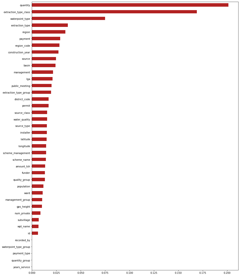
Feature importances

Feature importances will show the feature in the data set that has the most influece on the accuracy score for the model.

n = len(X_train.columns)
figsize = (15,20)

importances = pd.Series(search.best_estimator_.feature_importances_, X_train.columns)

top_n = importances.sort_values()[-n:]
plt.figure(figsize=figsize)
top_n.plot.barh(color='firebrick');

Feature-Importances

Model Permutations with ELI5

This niffty little python library will take feature importances and then determine how each feature is weighted.

permuter = PermutationImportance(search, scoring='accuracy', cv='prefit',
                     n_iter=2, random_state=42)

permuter.fit(X_val, y_val)

Weight	Feature
0.1065 ± 0.0009	quantity
0.0268 ± 0.0013	waterpoint_type
0.0212 ± 0.0048	payment
0.0208 ± 0.0005	construction_year
0.0169 ± 0.0017	latitude
0.0158 ± 0.0036	extraction_type
0.0149 ± 0.0002	longitude
0.0125 ± 0.0022	population
0.0110 ± 0.0034	source
0.0089 ± 0.0025	installer
0.0087 ± 0.0009	lga
0.0075 ± 0.0004	ward
0.0070 ± 0.0013	extraction_type_class
0.0066 ± 0.0025	region_code
0.0065 ± 0.0033	scheme_name
0.0065 ± 0.0007	funder
0.0060 ± 0.0007	gps_height
0.0047 ± 0.0028	amount_tsh
0.0044 ± 0.0000	basin
0.0041 ± 0.0000	management
0.0041 ± 0.0011	district_code
0.0036 ± 0.0007	extraction_type_group
0.0031 ± 0.0000	public_meeting
0.0030 ± 0.0002	region
0.0030 ± 0.0007	scheme_management
0.0018 ± 0.0013	permit
0.0015 ± 0.0027	id
0.0013 ± 0.0008	subvillage
0.0009 ± 0.0003	wpt_name
0.0009 ± 0.0013	management_group
0.0009 ± 0.0004	source_type
0.0007 ± 0.0002	water_quality
0.0007 ± 0.0013	source_class
0.0001 ± 0.0001	num_private
0.0001 ± 0.0004	quality_group
0 ± 0.0000	recorded_by
0 ± 0.0000	waterpoint_type_group
0 ± 0.0000	payment_type
0 ± 0.0000	quantity_group
0 ± 0.0000	years_service

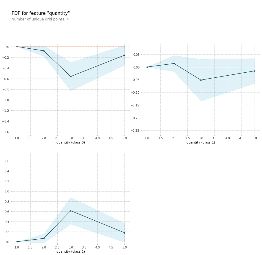
Last, we have some Partial Dependence Plots

Here is a single feature for water quantity PDP plot. The three classes represented in the plot are ‘Functional’, ‘Functional Needds Repair’, and ‘Non-Functional’ respectfully.

from pdpbox.pdp import pdp_isolate, pdp_plot

feature= 'quantity'
isolated = pdp_isolate(model=search, dataset=X_test, model_features=X_test.columns, feature=feature)

pdp_plot(isolated, feature_name=feature);

PDP-plot

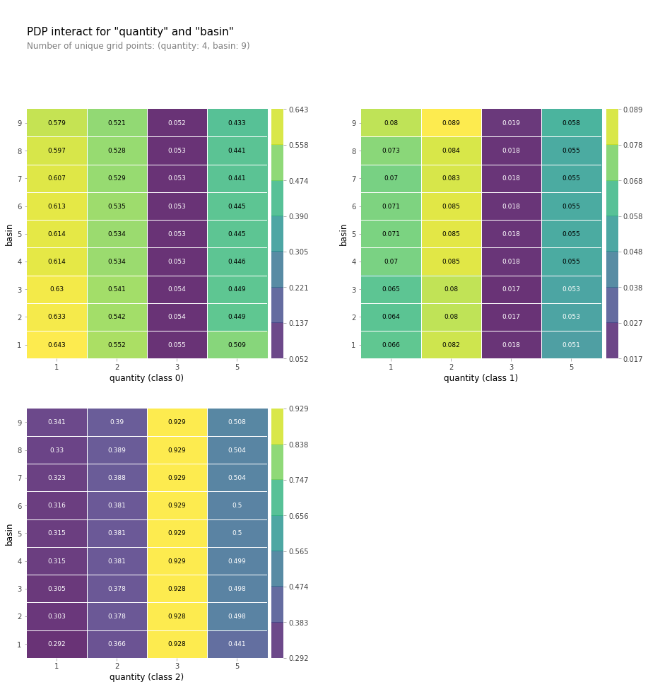
Partial Depedence Plot with Two Features

One final Partial Dependence Plot with the features of ‘qunatity’ and ‘basin’.

2 Features PDP

Conclusion

This challenge taught me alot about how important it that the water pumps in Tanzania are and that doing crazy amounts of feature engineering is always neccessary.

This dataset seemed to have a fair amount of NaN values. There also seemed to be additional values that looked like would result in a fair amount of outlier data and skewing of the data but it appears that XGBoost did a good job of not letting those hurdles to get in the way of finding a good accuracy score.

Thank you for taking the time to join me in my endeavor. My next project will be a Data Science Engineering one in which I am super excited about.

Predictive Modeling Kaggle Challenge

Tanzanian Water Pump Functionality Predictions

Predictive Modeling Kaggle Challenge

Tanzanian Water Pump Functionality Predictions

Purpose

Tanzanian Water Pump Kaggle Challenge Overview

Predict which water pumps are faulty.

Importing the Data and an Overloaded Toolbox

Examming the Dataset

First Baseline Model Prediction

XGBoost Classification with RandomizedSearchCV

Second Baseline Model Prediction

XGBoost Classification on Test Train Split Dataset with RandomizedSearchCV.

A Fun Little Confusion Matrix on the Prediction Model for Clarification.

Third Cleaned Data Model Prediction

Overdone Cleaning Funcion.

Cleaning Training Data

Cleaning Test

XGBoost Classification on Test Train Split Dataset with GridSearchCV and adjusted Hyper-parameters

Hey! Here is Another Model Confusion Matrix for Some More Clarification.

Here Are Some Fun but Simple Visualizations for Your Pleasure.

Feature importances

Model Permutations with ELI5

Last, we have some Partial Dependence Plots

Partial Depedence Plot with Two Features

Conclusion